Case 4: Reflecting wall and moving antennas

Ray tracing

Continuing from the previous example, now we let the receive antenna move towards the wall at the speed \(v\).

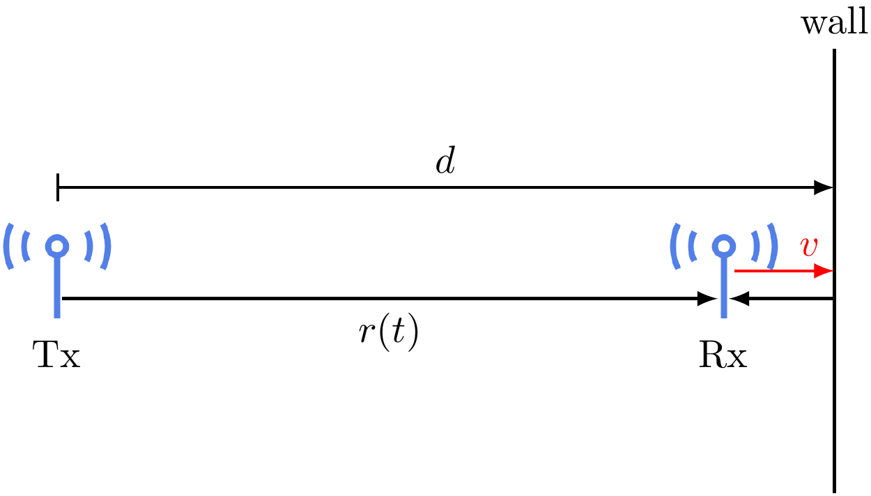
We need to update the time-varying distance between the two antennas as \(r(t) = r_0 + vt\). Using the same ray tracing method, we can calculate the received signal as \[ E_r(f,t) = \frac{\alpha \cos 2 \pi f \left[(1-v/c) t - r_0 / c\right]}{r_0+vt} - \frac{\alpha \cos 2 \pi f \left[(1+v/c)t + (r_0-2d)/c\right]}{2d-r_0-vt}. \]

Now assume that the denominators in the above equations are almost the same, namely \(r_0+vt \approx 2d - r_0 - vt\). This is true when the receive antenna is close to the wall. Then using the trigonometric identity \(\cos\theta - \cos\psi = 2 \sin\frac{\theta+\psi}{2} \sin\frac{\psi-\theta}{2}\), we have \[ E_r(f,t) \approx \frac{2 \alpha \sin 2 \pi f \left[(v/c) t + (r_0-d) / c\right] \sin 2 \pi f \left(t-d/c\right)}{r_0+vt}. \]

We can see that the receive signal is the product of two sinusoids. One sinusoid has the same frequency \(f\) as the transmit signal, while the other has a much lower frequency \(f(v/c)\), since the moving speed \(v\) of the antenna is much slower than the speed of light. For example, at a high moving speed of 40 miles/h (or about 60 km/h) and a frequency of \(f=3\) GHz, we have \(f(v/c) = 600\) Hz, which is much smaller than the carrier frequency.

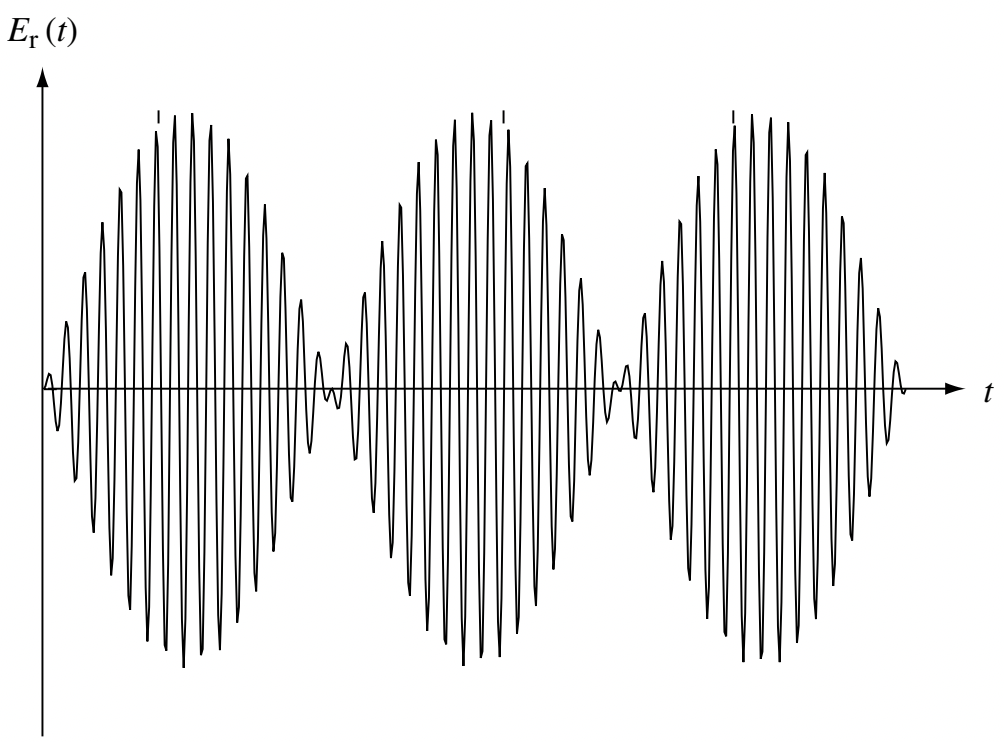
As illustrated above, the envelop of the receive signal varies at a low frequency of \(f(v/c)\), while the signal oscillates at the frequency \(f\) within the envelope.

Doppler spread and coherence time

From the graph of the received signal, we can see that it oscillates between strong and weak at a frequency of \(f(v/c)\). This frequency is closely related to Doppler shift. Specifically, due to the movement of the receive antenna, the signal from the line-of-sight path has a frequency of \(f(1-v/c)\), experiencing a Doppler shift of \(D_1 = -fv/c\), and the signal from the reflected path has a frequency of \(f(1+v/c)\), experiencing a Doppler shift of \(D_2 = +fv/c\). The difference between the Doppler shifts is defined as Doppler spread, namely \[ D_s \triangleq D_2 - D_1. \] In other words, the received signal oscillates at a frequency that equals half of the Doppler spread, namely \(f(v/c) = D_s/2\).

Since the strength of the received signal oscillates at the frequency \(f(v/c)\), the period of the oscillation is \(c / (fv)\). So the time it takes for the signal strength to go from the peak to the valley is \[ c / (4fv), \] which is called coherence time.

If you recall, we have defined the coherence distance in the previous example \[ \Delta x_c \triangleq \frac{\lambda}{4} = \frac{c}{4f}. \] We can see that the coherence time is \(c / (4fv) = \Delta x_c / v\). So the coherence time is exactly the time for the antenna to travel the coherence distance! Now we have these definitions in a full circle.

Take-away

Moving antennas result in Doppler spread, which is inversely proportional to the coherence time. The coherence time is the time for the antenna to travel the coherence distance.

Within the coherence time, we can consider the channel as almost constant.